Implementation

Since the effects of compressibility on performance proved interesting, the program used to test the performance of this algorithm was written with the ability to generate arrays with semi-random contents, but controllable compressibility. This was done by calculating the value of each array element by taking the random modulus of a low number, so that a non-deterministic but controllable number of data points had the same value (i.e. any time the random number was greater than the chosen low number, the result was the chosen low number). For example, the formula (k+1)-(k+1)%(rand()+1) can be used, where k is a variable which is incremented after each test run. For lower values of k, there is a lower probability that rand() will return a number is less than k, thus a greater probability that the above expression will evaluate to 0. As the value of k increases, the arrays generated have more non-zero elements, so they become less compressible on average. Each subsequent semi-random array is less compressible than the one used in the previous run. Since the compressibility of the data produced does not have a linear dependence on k, expressions with powers or exponentials of k were often used in place of just k for test runs. Compression trials could then be run in a loop, where the loop index k

$$\left\vert \begin{array}{cccccccccccccccc} 0 & 0 & 0 & 0 & 0 ... ... & 0 & 0 & 0 & 314 & 0 & 0 & 0 & 0 \\ \end{array} \right\vert$$

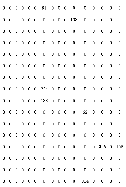
was incremented from 0 to 1000. The result is a record of compression times for arrays with compressibilities more or less evenly distributed from 0 to 1. The following 16x16 array was generated using this method.
This data can be mapped to a 4 level quadtree, as shown in Figure 17. The numbers at various nodes in the tree represent the value of every leaf below that point. Since the first 64 values are 0, a large 0 is on the left side of the figure to represent all the leaf values in that branch.

  

Figure 17: 256 element array mapped into a quadtree.

Compressed and represented as a string with sizes and values, the above array becomes the following 55 size-value pairs:
64-0 16-0 16-0 16-0 1-0 1-0 1-0 1-395 4-0 4-0 4-0 1-0 1-31 1-0 1-0 1-0 1-0 1-128 1-0 4-0 4-0 4-0 4-0 4-0 1-0 1-244 1-0 1-0 1-0 1-138 1-0 1-0 4-0 4-0 4-0 16-0 16-0 16-0 4-0 1-0 1-0 1-62 1-0 4-0 4-0 1-0 1-0 1-0 1-108 4-0 4-0 1-0 1-0 1-314 1-0
Using integer pairs to represent a compressed tree uses a lot of unnecessary space, and can be condensed quite a bit. For instance, if the tree height is less than 16 (a 65536 x 65536 array, or 16GB of data) the size component of the size-value pairs can be encoded as a tree height and a series of hex digits representing the level of the tree below which all numbers are the same. Or in terms of number of digits represented, the digits signify four raised to that number values, e.g. a 3 would signify a three level tree with the same value at each of its leaves, which could be 64 0s. So the size-value pair 64-0, using two 8 byte integers, would condense to a 3 in the encoded size part, taking up 4 bits, and 0 for the value, represented by 8 bytes. Not counting an initial 4 bits for the tree height, this encoding reduces the size by 5/8. In the example, this would result in the following 28 bytes:
43222000011100000000111110000000011122210000110000111111
So the total compression would be from 1024 bytes (256 integers x 4 bytes/integer) to 248 bytes (55 integers x 4 bytes/integer + 28 byte tree description), or a 76% reduction in size.